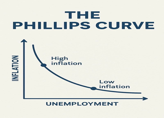
What is Phillips Curve

Definition: An economic concept demonstrating an inverse relationship between inflation and unemployment.
The Mechanism: Lower unemployment → higher aggregate wage income → increased consumer demand → higher prices (demand-pull inflation).
The Inverse: Higher unemployment reduces aggregate demand, leading to stable or declining inflation.

Origin: Formulated by economist A.W. Phillips in 1958.
Data Source: Based on an empirical analysis of UK unemployment and money wage rates from 1861 to 1957.
Evolution: Originally focused on wage inflation, later adapted by mainstream economists to apply to general price inflation.
Paradigm Shift: Widely accepted in the 1960s but faced a major theoretical crisis during the 1970s Stagflation, which contradicted its core premise.

Short-Run Phillips Curve (SRPC): A downward-sloping curve indicating a direct policy trade-off—achieving lower unemployment requires tolerating higher inflation.
Expectations-Augmented Phillips Curve: Propounded by Milton Friedman, it argues that public anticipation of future inflation alters wage demands and pricing behavior.
Long-Run Phillips Curve (LRPC): A vertical line indicating no trade-off in the long term. The economy naturally settles at the Natural Rate of Unemployment (NAIRU), regardless of the inflation rate.

Stagflation Blindspot: Completely fails to explain stagflation—a scenario of simultaneous high inflation, high unemployment, and stagnant growth.
Ignores Supply Shocks: Fails to account for inflation driven by external supply-side factors (e.g., crude oil price spikes, wars, or supply chain disruptions).
Long-Run Invalidity: Proves that central banks cannot permanently lower unemployment simply by artificially inflating the economy.
Role of Expectations: The traditional model underestimates how rational economic agents adapt their financial behavior to anticipated inflation.

Monetary Policy Guide: Serves as a vital analytical tool for central banks (like the RBI) to calibrate policy rates (repo rate).
Dual Mandate Balancing: Helps policymakers manage the constant trade-off between containing inflation and stimulating employment generation.
Short-Term Economic Management: Despite long-term flaws, it remains highly effective for tracking short-run macroeconomic dynamics and aggregate demand pressures.

While the Phillips Curve effectively models short-term trade-offs between inflation and unemployment, its failure to account for stagflation limits its long-term utility. Consequently, policymakers must look beyond this traditional framework and integrate robust supply-side interventions to ensure sustainable, non-inflationary economic growth.

1. Laffer Curve

Relationship: Tax rates versus Total tax revenue collection.
Trajectory: Inverted U-shaped curve.
Core Principle: Tax revenue increases with rising tax rates up to an “optimal rate.” Beyond this threshold, punitive rates disincentivize work, investment, and production, ultimately reducing total tax receipts.
Significance: Guides fiscal policy to set tax rates that maximize government revenue without distorting economic activity.

2. Lorenz Curve

Relationship: Cumulative percentage of population versus Cumulative percentage of national income/wealth.
Trajectory: Convex curve plotted against a straight 45-degree “Line of Perfect Equality.”
Core Principle: The further the curve sags away from the 45-degree line, the higher the degree of wealth or income inequality.
Significance: Serves as the primary graphical basis for deriving the Gini Coefficient to quantify national economic disparities.

3. Kuznets Curve

Core Principle: Income inequality inherently worsens during early stages of industrialization/development, plateaus, and systematically declines as the economy matures and welfare distribution improves.
Significance: Central to development economics when evaluating the trade-offs between rapid GDP expansion and social equity.

4. Engel Curve

Relationship: Household income level versus Quantity demanded of a specific commodity.

Upward-sloping: For normal and luxury goods (consumption rises as income increases).

Downward-sloping: For inferior goods (consumption falls as income increases).

Significance: Foundational microeconomic tool used to analyze consumer spending behavior, standard of living shifts, and demand elasticities.

5. Rahn Curve

Relationship: Government expenditure (as a % of GDP) versus Economic growth rate.
Trajectory: Inverted U-shaped curve.
Core Principle: Moderate public spending catalyzes growth by establishing infrastructure, rule of law, and basic public goods. Beyond the optimal scale, excessive state spending reduces growth via taxation burdens, bureaucratic inefficiencies, and the crowding-out of private capital.
Significance: Informs fiscal authorities on determining the optimal size and limits of public sector expenditure.

6. Beveridge Curve

Relationship: Unemployment rate versus Job vacancy rate in an economy.
Trajectory: Downward-sloping curve.
Core Principle: High unemployment corresponds with low job vacancies (economic downturns), and vice versa. An outward shift of the entire curve indicates rising structural labor market frictions, such as skill mismatches.
Significance: Assesses labor market efficiency, distinguishes cyclical from structural unemployment, and evaluates job-creation policies.

7. J-Curve

Relationship: Currency depreciation/devaluation versus Trade balance over time.
Trajectory: J-shaped trajectory.
Core Principle: Following currency depreciation, a nation’s trade balance initially deteriorates because import payments adjust immediately while export volumes take time to respond. As export price-competitiveness takes effect, trade balances steadily recover and improve.
Significance: Key reference for foreign exchange interventions, trade policy design, and managing current account deficits (CAD).

This Concept has been discussed in the following article:

A Decade of Inflation Targeting: Evaluating India’s Monetary Compass

Latest Articles